import pandas as pd
import numpy as np
import os
import matplotlib.pyplot as plt
import matplotlib.patches as mpatches
from matplotlib import colors
import xarray as xr
import rioxarray as rioxr
import geopandas as gpd
import pystac_client
import planetary_computer
import contextily as cx
from pystac_client import Client  # To access STAC catalogs
import planetary_computer  # To sign items from the MPC STAC catalog
from IPython.display import Image # To nicely display imagesBy Amanda Overbye
This notebook performs an analysis of the Biodiversity Intactness Index (BII) for Maricopa County (Phoenix) by comparing BII values in 2017 and 2020. We use the io-biodiversity dataset provided by Impact Observatory and Vizzuality and clip it to the boundary of Maricopa County. You can find the Github repository for it here
Highlights
Geospatial Data Handling:
- Loading and manipulating geospatial data using libraries like geopandas and rioxarray.
- Filtering geographic data for specific regions (e.g., Maricopa County, Phoenix) using shapefiles.
- Reprojecting coordinate reference systems (CRS) for compatibility.
Data Access and Integration:
- Accessing remote datasets (Biodiversity Intactness Index) via the Microsoft Planetary Computer using the pystac_client library.
- Searching and retrieving specific datasets using spatial queries (bounding boxes) and time ranges.
Raster Data Processing:
- Working with raster data (e.g., BII values) and applying geospatial analysis, such as clipping and thresholding.
Data Visualization:
- Creating maps and visualizing spatial data, including the use of color gradients, legends, and basemaps for better interpretation.
Data
o-biodiversity DatasetThe io-biodiversity dataset, available on Microsoft’s Planetary Computer, contains Biodiversity Intactness Index (BII) values for the years 2017–2020. The BII measures the abundance of species in an area, offering insights into global biodiversity health. This dataset, provided by Impact Observatory and Vizzuality, is available at a 100-meter resolution and can be accessed through the pystac_client library for specific geographic areas and time periods.
Shapefile (tl_2016_04_tract.shp)The 2020 TIGER/Line shapefile for Arizona, provided by the US Census Bureau, contains detailed geographic boundaries for Census subareas (Cousubs) within the state. This dataset is useful for analyzing regional demographic, social, and economic data at a granular geographic level.
References
Microsoft Planetary Computer, STAC Catalog. Biodiversity Intactness. [Dataset]. https://planetarycomputer.microsoft.com/dataset/io-biodiversity. Accessed 7 December, 2024.
United States Census Bureau. 2024. Arizona County TIGER/Line Shapefiles. [Dataset]. United States Census Bureau. https://www.census.gov/geographies/mapping-files/time-series/geo/tiger-line-file.html. Accessed 7 December, 2024.
1. Setup and Libraries
2. Load Subdivision Shapefile
# Load subdivision shapefile (county subdivisions for Arizona)
subdivision = gpd.read_file('data/subdivision/tl_2024_04_cousub.shp')

# Print first few rows to check the data
print(subdivision.head())
STATEFP COUNTYFP COUSUBFP COUSUBNS GEOID GEOIDFQ \
0 04 005 91198 01934931 0400591198 0600000US0400591198
1 04 005 91838 01934953 0400591838 0600000US0400591838
2 04 005 91683 01934950 0400591683 0600000US0400591683
3 04 023 92295 01934961 0402392295 0600000US0402392295
4 04 023 92550 01934966 0402392550 0600000US0402392550
NAME NAMELSAD LSAD CLASSFP MTFCC FUNCSTAT \
0 Flagstaff Flagstaff CCD 22 Z5 G4040 S
1 Kaibab Plateau Kaibab Plateau CCD 22 Z5 G4040 S
2 Hualapai Hualapai CCD 22 Z5 G4040 S
3 Nogales Nogales CCD 22 Z5 G4040 S
4 Patagonia Patagonia CCD 22 Z5 G4040 S
ALAND AWATER INTPTLAT INTPTLON \
0 12231962349 44576380 +35.1066122 -111.3662507
1 7228864156 29327221 +36.5991097 -112.1368033
2 2342313339 3772690 +35.9271665 -113.1170408
3 1762339489 2382710 +31.4956020 -111.0171332
4 1439560139 685527 +31.5664619 -110.6410279
geometry
0 POLYGON ((-112.13370 35.85596, -112.13368 35.8...
1 POLYGON ((-112.66039 36.53941, -112.66033 36.5...
2 POLYGON ((-113.35416 36.04097, -113.35416 36.0...
3 POLYGON ((-111.36692 31.52136, -111.36316 31.5...
4 POLYGON ((-110.96273 31.68695, -110.96251 31.6... 3. Filter for Maricopa County (Phoenix Area)
# Filter for Maricopa County (Phoenix area)
maricopa = subdivision[subdivision['NAME'] == "Phoenix"]
4. Access STAC Catalog and Biodiversity Data
# Access the STAC catalog for biodiversity data
catalog = Client.open(
    "https://planetarycomputer.microsoft.com/api/stac/v1",
    modifier=planetary_computer.sign_inplace,
)

# Access the 'io-biodiversity' collection
biodiversity = catalog.get_child('io-biodiversity')
5. Defining the Temporal And Geographic Ranges
# Pheonix bounding box
bbox = {
    "type": "Polygon",
    "coordinates": [
        [
            [-112.826843, 32.974108],  # Bottom-left corner
            [-112.826843, 33.863574],  # Top-left corner
            [-111.184387, 33.863574],  # Top-right corner
            [-111.184387, 32.974108],  # Bottom-right corner
            [-112.826843, 32.974108],  # Closing the polygon
        ]
    ],
}


# Define time range for 2020 and 2017
time_range_2020 = "2020-01-01/2020-12-31"
time_range_2017 = "2017-01-01/2017-12-31"
6. Catalog Search and Retrieve Data for 2020 and 2017
# Catalog search for 2020 with time range
search_2020 = catalog.search(
    collections=["io-biodiversity"],
    intersects=bbox,  # Your bounding box
    datetime=time_range_2020  # Using time range for 2020
)
item_2020 = search_2020.item_collection()[0]  # First item in the collection

# Catalog search for 2017 with time range
search_2017 = catalog.search(
    collections=["io-biodiversity"],
    intersects=bbox,  # Your bounding box
    datetime=time_range_2017  # Using time range for 2017
)
item_2017 = search_2017.item_collection()[0]  # First item in the collection
8. Load Data for 2020 and 2017
# Loading in the data
rast_2020 = rioxr.open_rasterio(item_2020.assets["data"].href)
rast_2017 = rioxr.open_rasterio(item_2017.assets["data"].href)
9. The Subdivision in Context
fig, ax = plt.subplots(figsize=(10, 10))

# Create face color and adjust alpha
fc = colors.to_rgba('mistyrose')
fc = fc[:-1] + (0.4,)

# Plot the `maricopa` GeoDataFrame
maricopa.to_crs(epsg=3857).plot(ax=ax, edgecolor="red", facecolor=fc)

# Add basemap
cx.add_basemap(ax, zoom=10, source=cx.providers.CartoDB.Voyager)

# Add legend
legend_patch = mpatches.Patch(color='mistyrose', label='Maricopa County')
ax.legend(handles=[legend_patch], loc='upper left', fontsize=10)

# Add title
ax.set_title("Maricopa County (Phoenix) - County Subdivisions", fontsize=16)

# Show the plot
plt.show()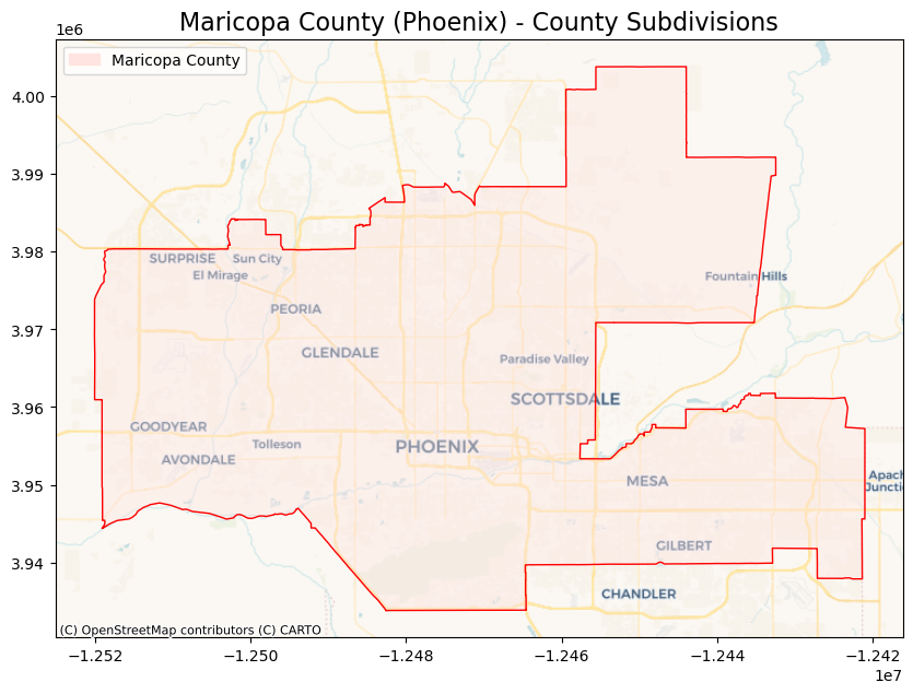
# Check CRS of the Maricopa GeoDataFrame
print(maricopa.crs)

# Reproject to match the biodiversity dataset CRS
maricopa = maricopa.to_crs("EPSG:4326")EPSG:4269# Filter for Phoenix subdivision (using the NAME column)
phoenix = maricopa[maricopa['NAME'] == "Phoenix"]10. Clip Raster Data to the Phoenix Boundary
# Clip the 2020 raster using the Phoenix geometry
phoenix_clip_2020 = rast_2020.rio.clip(phoenix.geometry)

# Clip the 2017 raster using the Phoenix geometry
phoenix_clip_2017 = rast_2017.rio.clip(phoenix.geometry)
11. Plot the Clipped Data for 2017 and 2020
# Plot the clipped raster with the Maricopa County shapefile boundary
fig, ax = plt.subplots()
phoenix_clip_2020.plot(ax=ax)
phoenix.plot(ax=ax, color=(0.1, 0.2, 0.5, 0.01), edgecolor="black")
plt.show()
# Plot the clipped raster with the Maricopa County shapefile boundary
fig, ax = plt.subplots()
phoenix_clip_2017.plot(ax=ax)
phoenix.plot(ax=ax, color=(0.1, 0.2, 0.5, 0.01), edgecolor="black")
plt.show()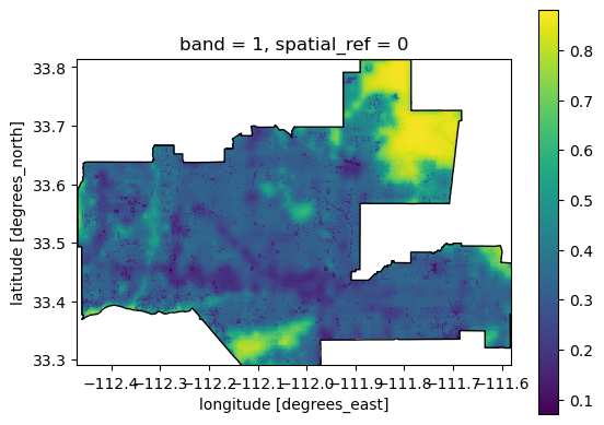
12. Calculate BII for Areas Above Threshold (≥ 0.75)
# Convert to boolean arrays for BII >= 0.75
bii_2020_high = (phoenix_clip_2020 >= 0.75).astype(int)
bii_2017_high = (phoenix_clip_2017 >= 0.75).astype(int)
# Find the total number of pixels for each year
total_pixels_2020 = bii_2020_high.count().item()
total_pixels_2017 = bii_2017_high.count().item()# Find count of pixels above 0.75 BII for each year
bii_pixels_2020 = bii_2020_high.values.sum()
bii_pixels_2017 = bii_2017_high.values.sum()# Calculate percentages
bii_pct_2020 = (bii_pixels_2020 / total_pixels_2020) * 100
bii_pct_2017 = (bii_pixels_2017 / total_pixels_2017) * 100print(f"In 2017, {round(bii_pct_2017, 2)}% of Phoenix County had a BII of at least 0.75")
print(f"In 2020, {round(bii_pct_2020, 2)}% of Phoenix had a BII of at least 0.75")In 2017, 4.18% of Phoenix County had a BII of at least 0.75
In 2020, 3.81% of Phoenix had a BII of at least 0.7513. Calculate BII Loss Between 2017 and 2020
# Calculate the difference in pixels above 0.75 from 2017 to 2020
diff_2017_2020 = bii_2017_high - bii_2020_high
# Set all that are not 1 to NA (pixels that fell below threshold)
loss_2017_2020 = diff_2017_2020.where(diff_2017_2020 == 1)14. Visualize BII Loss
# Create map
fig, ax = plt.subplots(figsize=(10, 10))
ax.axis('off')

# Plot BII for 2020
phoenix_clip_2020.plot(ax=ax, cmap='Greens', cbar_kwargs={'orientation': 'horizontal', 'label': 'BII for 2020'})

# Plot BII loss
loss_2017_2020.plot(ax=ax, cmap='brg', add_colorbar=False)

# Plot Maricopa boundary
phoenix.plot(ax=ax, color='none', edgecolor='black', linewidth=0.75)

# Add legend
legend = [mpatches.Patch(facecolor='red', label='Area with BII ≥ 0.75 lost from 2017 to 2020')]
ax.legend(handles=legend, loc=(0.25, -0.2))

# Set title
ax.set_title("Biodiversity Intactness Index (BII)\ In Phoenix Subdivisions")

# Show plot (no saving)
plt.show()
This map shows the Biodiversity Intactness Index (BII) for Maricopa County, which includes the Phoenix metropolitan area, in 2020. The BII is represented by a green color gradient, with darker shades indicating higher biodiversity intactness.
The red highlighted areas are locations that experienced significant BII loss between 2017 and 2020 - their BII dropped below 0.75 during this time period, indicating major biodiversity degradation.
References
Microsoft Planetary Computer, STAC Catalog. Biodiversity Intactness. [Dataset]. https://planetarycomputer.microsoft.com/dataset/io-biodiversity. Accessed 7 December, 2024.
United States Census Bureau. 2024. Arizona County TIGER/Line Shapefiles. [Dataset]. United States Census Bureau. https://www.census.gov/geographies/mapping-files/time-series/geo/tiger-line-file.html. Accessed 7 December, 2024.